numpy.geomspace#

numpy.geomspace(start, stop, num=50, endpoint=True, dtype=None, axis=0)[source]#

Return numbers spaced evenly on a log scale (a geometric progression).

This is similar to logspace, but with endpoints specified directly. Each output sample is a constant multiple of the previous.

Changed in version 1.16.0: Non-scalar start and stop are now supported.

Parameters

startarray_like: The starting value of the sequence.
stoparray_like: The final value of the sequence, unless endpoint is False. In that case, num + 1 values are spaced over the interval in log-space, of which all but the last (a sequence of length num) are returned.
numinteger, optional: Number of samples to generate. Default is 50.
endpointboolean, optional: If true, stop is the last sample. Otherwise, it is not included. Default is True.
dtypedtype: The type of the output array. If dtype is not given, the data type is inferred from start and stop. The inferred dtype will never be an integer; float is chosen even if the arguments would produce an array of integers.
axisint, optional: The axis in the result to store the samples. Relevant only if start or stop are array-like. By default (0), the samples will be along a new axis inserted at the beginning. Use -1 to get an axis at the end.

New in version 1.16.0.

Returns

samplesndarray: num samples, equally spaced on a log scale.

See also

logspace: Similar to geomspace, but with endpoints specified using log and base.
linspace: Similar to geomspace, but with arithmetic instead of geometric progression.
arange: Similar to linspace, with the step size specified instead of the number of samples.

Notes

If the inputs or dtype are complex, the output will follow a logarithmic spiral in the complex plane. (There are an infinite number of spirals passing through two points; the output will follow the shortest such path.)

Examples

>>> np.geomspace(1, 1000, num=4)
array([    1.,    10.,   100.,  1000.])
>>> np.geomspace(1, 1000, num=3, endpoint=False)
array([   1.,   10.,  100.])
>>> np.geomspace(1, 1000, num=4, endpoint=False)
array([   1.        ,    5.62341325,   31.6227766 ,  177.827941  ])
>>> np.geomspace(1, 256, num=9)
array([   1.,    2.,    4.,    8.,   16.,   32.,   64.,  128.,  256.])

Note that the above may not produce exact integers:

>>> np.geomspace(1, 256, num=9, dtype=int)
array([  1,   2,   4,   7,  16,  32,  63, 127, 256])
>>> np.around(np.geomspace(1, 256, num=9)).astype(int)
array([  1,   2,   4,   8,  16,  32,  64, 128, 256])

Negative, decreasing, and complex inputs are allowed:

>>> np.geomspace(1000, 1, num=4)
array([1000.,  100.,   10.,    1.])
>>> np.geomspace(-1000, -1, num=4)
array([-1000.,  -100.,   -10.,    -1.])
>>> np.geomspace(1j, 1000j, num=4)  # Straight line
array([0.   +1.j, 0.  +10.j, 0. +100.j, 0.+1000.j])
>>> np.geomspace(-1+0j, 1+0j, num=5)  # Circle
array([-1.00000000e+00+1.22464680e-16j, -7.07106781e-01+7.07106781e-01j,
        6.12323400e-17+1.00000000e+00j,  7.07106781e-01+7.07106781e-01j,
        1.00000000e+00+0.00000000e+00j])

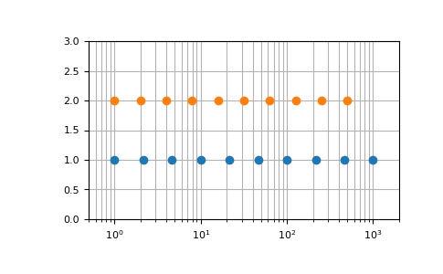
Graphical illustration of endpoint parameter:

>>> import matplotlib.pyplot as plt
>>> N = 10
>>> y = np.zeros(N)
>>> plt.semilogx(np.geomspace(1, 1000, N, endpoint=True), y + 1, 'o')
[<matplotlib.lines.Line2D object at 0x...>]
>>> plt.semilogx(np.geomspace(1, 1000, N, endpoint=False), y + 2, 'o')
[<matplotlib.lines.Line2D object at 0x...>]
>>> plt.axis([0.5, 2000, 0, 3])
[0.5, 2000, 0, 3]
>>> plt.grid(True, color='0.7', linestyle='-', which='both', axis='both')
>>> plt.show()

numpy.logspace

numpy.meshgrid